Precalc with Python 2.0
by Kirby Urner
First posted: Sept 10, 2000
Last modified: Sept 25, 2000
The source code below is a single module, precalc.py, and is available minus the HTML markup tags and interpolated text, i.e. in a form suitable for running directly under Python 2.0 or above. I recommend students use the IDLE graphical interface, or similar shell, in order to take advantage of a color-coded command line interface. Both Windows and Linux have IDLE -- I'm still discovering what's out there for the iMac (apparently Guido's brother Jan has done some valuable work in this area -- Guido being Python's principal inventor and designer of course).
At the time of this writing, Python 2.0 is still in beta. All the general ideas could be implemented in an earlier Python, however I've gone with 2.0 because some of the new zip(sequence...) and list comprehension syntax -- [function(x) for x in sequence] -- is especially useful for streamlining the code.
The precalc.py module stands alone conceptually (given some background in Python itself), but does depend on other modules in support of its graphing functions. Python's native support for the Tk cross-platform graphical system has been supplanted by Povray in a lot of my writings, although I have done some work with the Tk canvas (I'm waiting for bug fixes in 2.0b2, before I share any of it -- see Python and Tkinter Programming by John E. Grayson for more on Python and Tk).
So I would recommend my Numeracy + Computer Literacy series as useful background for both Python and these Povray-related classes and functions.
"""
precalc:  module for helping teachers help kids grok calculus
Relevant documentation posted to edu-sig@python.org

Last updated: Sept. 25, 2000

Thanks to David Scherer, Dustin Mitchell, and Jeff Cogswell
for suggestions
"""

import povray, functions, string
from coords import Vector
from math import *
from functions import mkdomain

defwiggle(function,input,epsilon=1e-10):
    """Accepts a function, value and returns delta f / delta x
    for small epsilon (default of 10^-10 may be overridden)
    """
    return (function(input+epsilon) - function(input))/epsilon
The wiggle function is analogous to the derivative at point input. A continuous function is passed as the first parameter, and a default epsilon gets used to "wiggle" the input value by epsilon, measuring the difference in function outputs against the tiny interval itself i.e. delta_f(x)/delta_x.
Note that in this case we expect the function to be passed as an algebraic rule, such that input and input+epsilon are meaningful as inputs, or members of the function's domain.
The runtotal function (below) is an inverse operation, analogous to the integral. Whereas the wiggle function takes snap shots of change per interval (change/delta_x), the runtotal function keeps a running total of changes for intervals (change * delta_x).
Here we don't expect an algebraic rule as input, but a function as a set of (domain,range) pairs. Successive domain values get averaged (avgx), as do successive range values (avgy), to give an accumulating total of avgy * increment at each avgx. The output of this function is a list pairing avgx with the corresponding running total values (i.e. the accumulation of products to this point).
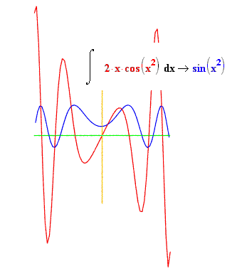
As you will see from the graphs below, the runtotal function, when run against the output of the wiggle function, gets us back to the original curve, albiet displaced vertically by some constant K. This should help students grasp the Fundamental Theorem and the fact that differentiation and integration are inverse operations.
defruntotal(function):
    """Accepts a function, returns (x, running total) pairs --
    analogous to definite integral
    """
    # initialize
    rtotal = 0
    output = []
    lastx,lasty = function[0]
    for x,y in function[1:]:
        avgy   = (lasty + y)/2.0        # average f(x)
        avgx   = (lastx + x)/2.0        # average x
        incre  = x - lastx              # domain increment
        rtotal = rtotal + (avgy * incre)
        output.append((avgx,rtotal))
        lastx  = x
        lasty  = y
    return output
Below is the function I use to "connect the dots" in Povray. It connects successive points in the input function with edges, generating a relatively smooth curve provided the domain values were close enough together to begin with.
defgraphit(myfunc, myfile):
    # draws function
    xaxislen = max( abs(myfunc[0][0]),abs(myfunc[-1][0]) )
    functions.xyzaxes(myfile,xaxislen)
    # draw edges between pairs of 3-tuples (x,y,z), z=0
    for p1,p2 in zip(myfunc,myfunc[1:]):
        v1,v2 = (p1[:]+(0,)),(p2[:]+(0,))
        myfile.edge(Vector(v1),Vector(v2))   # draw edge between the two
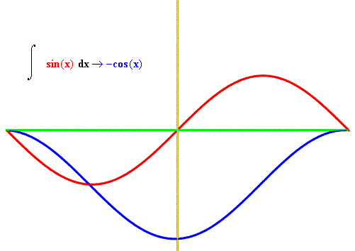
The next three example methods make use of the graphit function to show how the output of a wiggled function is itself a function. In the first example, the red cuve is a standard sine wave, whereas the blue curve is the wiggled version, or derivative function -- the cosine wave.
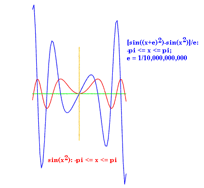
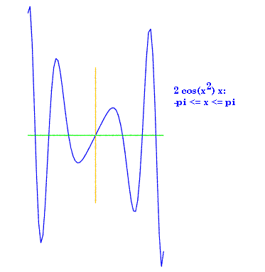
In the second and third examples, we use a slightly more complicated function and show that the algebraic derivative gives the same curve as the analogous "wiggle derivative" obtained by means of discrete math.
defwiggle1(): dom = mkdomain(-pi,pi,0.1) # note step by 0.1 rng = [wiggle(sin,x) for x in dom] func = zip(dom,rng) sine = zip(dom,[sin(x) for x in dom]) # sine function drawfile = povray.Povray("wiggle1.pov",cf=15,cx=0,cy=0) graphit(func,drawfile) # accepts list of [(dom,rng)] pairs drawfile.cylcolor = "Red" drawfile.sphcolor = "Red" graphit(sine,drawfile) drawfile.close()defG(x): return sin(x**2) defderivG(x): return 2*cos(x**2)*x deflinear(x): return 2*x defwiggle2(): dom = mkdomain(-pi,pi,0.1) # note step by 0.1 funcG = zip(dom,[G(x) for x in dom]) wiggleG = zip(dom,[wiggle(G,x) for x in dom]) drawfile = povray.Povray("wiggle2.pov",cf=38,cx=0,cy=0) # [3] graphit(wiggleG,drawfile) # accepts list of [(dom,rng)] pairs drawfile.cylcolor = "Red" drawfile.sphcolor = "Red" graphit(funcG,drawfile) drawfile.close()
defwiggle3():
    dom  = mkdomain(-pi,pi,0.1)  # note step by 0.1
    derivfuncG = zip(dom,[derivG(x) for x in dom])
    drawfile = povray.Povray("wiggle3.pov",cf=38,cx=0,cy=0) # [3]
    graphit(derivfuncG,drawfile)   # accepts list of [(dom,rng)] pairs
    drawfile.close()
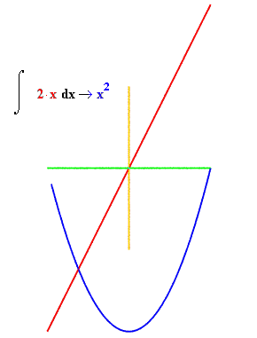
The three accumulate functions test our runtotal function by passing it (domain, range) pairs. In the first example, we use a simple linear function, f(x) = 2x. The returned function is parabolic, as expected. In the second example, we use the same algebraic derivG(x) function used in wiggle3 as input, and get back a curve that looks a lot like the original G(x) -- although displaced by K.
Note that whereas wiggle uses a tiny epsilon to obtain a smattering of delta_f/delta_x readings for a function, the running total approach spans wider gaps by connecting the dots between successive input function domain values when deriving avgx. This is because runtotal is designed to operate on sets of coordinate pairs, not an algebraic rule, i.e. there's no way to sample at a higher frequency than what the input function provides.
Also, although we could push the sample rate to a very high frequency when using wiggle, and have points only separated by epsilon instead of 0.1 as in the above examples, in practice we're satisfied with a relatively smooth curve close to the threshold of screen resolution, and so do not consider it necessary to burden runtotal with such a long list of input values as this would require.
defaccumulate1():
    dom = mkdomain(-2,2,0.1)
    f = zip(dom,[linear(x) for x in dom])
    intf = runtotal(f)
    drawfile = povray.Povray("int1.pov",cf=25,cx=0,cy=0) # [3]
    graphit(intf,drawfile)
    drawfile.cylcolor = "Red"
    drawfile.sphcolor = "Red"
    graphit(f,drawfile)
    drawfile.close()
defaccumulate2():
    dom  = mkdomain(-pi,pi,0.1)  # note step by 0.1
    derivfuncG = zip(dom,[derivG(x) for x in dom])
    integral = runtotal(derivfuncG)
    drawfile = povray.Povray("int2.pov",cf=38,cx=0,cy=0) # [3]
    graphit(integral,drawfile)
    drawfile.cylcolor = "Red"
    drawfile.sphcolor = "Red"
    graphit(derivfuncG,drawfile)
    drawfile.close()
defaccumulate3():
    dom  = mkdomain(-pi,pi,0.1)  # note step by 0.1
    sine = zip(dom,[sin(x) for x in dom]) # sine function
    integral = runtotal(sine)
    drawfile = povray.Povray("int3.pov",cf=15,cx=0,cy=0) # [3]
    graphit(integral,drawfile)
    drawfile.cylcolor = "Red"
    drawfile.sphcolor = "Red"
    graphit(sine,drawfile)
    drawfile.close()
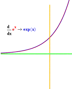
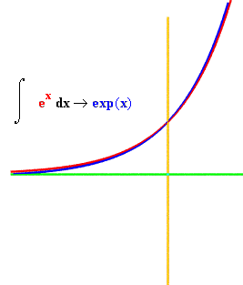
In the final two examples, we study the special relationship of the exponential function, i.e. Euler's number e raised to the x, or f(x) = e**x (** is Pythonic for "raised to the power of"). This function, sent through wiggle, returns another, identical function. In other words, this function is identical with its derivative function. Likewise, runtotal returns the same function, although, as the curves show, the fit isn't quite as close, because of the value averaging that goes on in these discrete math approximations.
defwiggle4():
    dom   = mkdomain(-3,1.2,0.1)  # note step by 0.1
    rng   = [wiggle(exp,x) for x in dom]
    deriv = zip(dom,rng)
    expf  = zip(dom,[exp(x) for x in dom]) # exponential function
    drawfile = povray.Povray("wiggle4.pov",cf=15,cx=0,cy=0)
    graphit(deriv,drawfile)   # accepts list of [(dom,rng)] pairs
    drawfile.cylcolor = "Red"
    drawfile.sphcolor = "Red"
    graphit(expf,drawfile)
    drawfile.close()

defaccumulate4():
    dom  = mkdomain(-3,1.2,0.1)  # note step by 0.1
    expf = zip(dom,[exp(x) for x in dom]) # e**x
    integral = runtotal(expf)
    drawfile = povray.Povray("int4.pov",cf=15,cx=0,cy=0) # [3]
    graphit(integral,drawfile)
    drawfile.cylcolor = "Red"
    drawfile.sphcolor = "Red"
    graphit(expf,drawfile)
    drawfile.close()
The Java applet below uses the analogy of a movie. Each frame captures a discrete difference in the sine function, with the blue numbers showing its values at the start and end of delta t (time interval). The red number in each frame shows the absolute difference between these start and stop values, while the black number is the difference per interval, i.e. diff/interval, analogous to df(t)/dt.
Click mouse to start/stop
Playing off this movie metaphor, I've packaged some of the same functionality provided by the above tools into a camera class.
What's especially useful about this class is it expects to get an algebraic rule as a character string, with x the variable. This allows a function to be passed from a text box or read from a file. Coming up with efficient syntax for this feature was a useful learning experience for me on the edu-sig e-list (my initial solution was pretty complicated compared to David's, and slow compared to Jeff's).
classcamera:
    """
    Accepts algebraic rule as text string in terms of variable x
    e.g. '2*x**2 - 3*x + 10' -- evaluates f(x) and/or f'(x) over
    the supplied domain (defined by low, high and step values)
    """

    def__init__(self,txtRule,low=-1,high=1,interval = 0.125,
                 epsilon=1e-10):
        self.interval = 0.125
        # turn text rule into a function
        self.rule = eval("lambda x : %s" % txtRule)
        self.dom = mkdomain(low,high,interval)

    defgety(self,x):
        # return f(x)
        return self.rule(x)

    defgetrange(self):
        # evaluate rule over entire domain
        return [self.gety(x) for x in self.dom]

    defgetderiv(self,x):
        # return approximate derivate for given x
        return wiggle(self.gety,x)

    defgetfunction(self):
        # return the function itself as a list of (domain,range) pairs
        return zip(self.dom,self.getrange())

    defgetmovie(self):
        # return approximate derivative over entire domain
        return zip(self.dom,[self.getderiv(x) for x in self.dom])
Relevant links:
- Source code (to graph, you also need modules in Python101.zip + Povray)
- Background re Python syntax on k12.ed.math -- [f(x) for x in seq], zip(seq,seq)
- Calculus Intro
- Algebraic Integrator from Wolfram Research
- Catenary page
- Numeracy + Computer Literacy series
- Computer language index
