Before we proceed with the construction of our enimga-class enciphering machine, let's pause to look at another example of a group.
As most books on group theory will tell you, we grow to appreciate the generic concept of groups by working with special case examples. Through this kind of experience, we develop our intuitions regarding the generalized, exceptionless principles at work in each case. Likewise, our faculties for thinking at this more generalized level grow and mature through studying examples. Mathematics assists us to ascend the "pyramid of generalizations", from a base of many examples to an apex of more unifying abstractions.
Once we're able to work at this more general level, our findings will inevitably apply to all the special cases. This is what philosopher R. Buckminster Fuller (1895 - 1983) termed the principle of synergetic advantage: thinking in terms of wholes in order to better appreciate the operations and organization of the parts (the special cases).
The example of a group we've been using so far consists of permutations. A permutation pairs elements such that each maps to another in the same set, and all are accounted for. Some elements may well map to themselves, but thus "fixing" an element nevertheless introduces a unique pairing, i.e. no other element will also map to the same paired value.
Multiplication, in the case of permutations, is a kind of composition of functions, wherein scramblings of the alphabet (or some other set, e.g. playing cards) are chained together, one after another. The outcome is yet another scrambling (closure property), plus every permutation has a unique inverse which "undoes the doing" of the first, reversing its effects (inverse property) -- the net effect being "no change" or the identity permutation (e.g. every letter maps to itself).
Residue Classes
The next example of a group we will consider consists of the set of positive integers relatively prime to some greater integer, with multiplication being a clock-like or "modulo" operation, wherein values "wrap around" in a circle of permitted values. It's this "wrapping around" which makes these groups finite.
class R:

    def __init__(self,val,n):
        self.v = val%n
        self.n = n

    def __mul__(self,m):
        """
        a*b = (a*b) mod n
        """
        return R(self.v * m.v, self.n)

    def __div__(self,m):
        return self * m.inv()
Another reason for looking at this new kind of group, as defined by the R-class (residue class), is its application to a whole other approach to enciphering. Our enigma-style system depends on two parties, the sender and recipient of the ciphertext, to set their rotors to the same initial permutations. These rotor settings constitute a private or secret key, which needs to be sent separately. If a 3rd party gets ahold of this private key, the security of the ciphertext is compromised.
In contrast, with public key cryptography, all the participants freely publish what are called public keys. There's no harm in someone knowing your public key, and, in fact, they have to know it if they're going to encipher a message to you. Paired with your public key, is a private one, which exists only on your end -- unlike the secret key for enigma-class machines, you don't ever need to transmit it.
The combination of both public and private keys unlocks a message encrypted with a public key. So only you can read text enciphered with your public key (because you and you alone possess the paired private key).
Let's recall
the essential properties of a group:
Closure,
Associativity,
Inverse and Neutral
(CAIN). In the case of
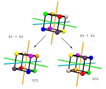
permutations, multiplication is not necessarily commutative, so
this was not an example of an Abelian group. For example, two
rotation permutations, if acting on copies of a cube as
>>> from rotations import Cube
>>> colors
{'H': 'Green', 'F': 'Pink', 'G': 'Violet', 'D': 'Yellow',
'E': 'Magenta', 'B': 'Blue', 'C': 'Orange', 'A': 'Red'}
>>> oc1 = Cube()  # identical cubes to start
>>> oc2 = Cube()
>>> oc1.rotate((oc1.pgroup[1] * oc1.pgroup[3])) # same permuations...
>>> oc1.pgroup[1]*oc1.pgroup[3]
Permutation: [('H', 'D'), ('F', 'C'), ('G', 'B'), ('E', 'A')]
>>> oc1.corners
['E', 'G', 'F', 'H', 'A', 'C', 'B', 'D']
>>> oc2.rotate((oc2.pgroup[3] * oc2.pgroup[1])) # ...but changed order
>>> oc2.pgroup[3]*oc2.pgroup[1]
Permutation: [('H', 'D'), ('F', 'B'), ('G', 'A'), ('E', 'C')]
>>> oc2.corners
['G', 'F', 'E', 'H', 'C', 'B', 'A', 'D']
Consider the number 20, and all positive integers below 20 which have no factors in common with 20 -- we say these integers are relatively prime, or coprime to 20.
>>> from ciphers import *
>>> relprimes(20)
[1, 3, 7, 9, 11, 13, 17, 19]
If two integers are relatively prime, this means their greatest commond divisor, or gcd, is 1. We have a rather simple method for finding the gcd, based on what we call Euclid's Algorithm, one of the oldest on record. This algorithm tries to divide a smaller into a larger number, and if there's a remainder, tries to divide the remainder into the smaller number, and so on, in a series of steps guarenteed to eventually reach a common divisor -- which may eventually turn out to be 1.
def gcd(a,b):
    """Return greatest common divisor using Euclid's Algorithm."""
    while b:
    a, b = b, a % b
    return a
Once the gcd is in place, it's a simple matter to simply iterate through the positive integers less than N (e.g. N=20) and find all those relatively prime to 20, i.e. gcd(x,20)==1. List comprehension syntax works well for this application:
def relprimes(n):
    """
    List integers 0 < i < n, such that i,n are coprime
    """
    return [x for x in range(1,n) if gcd(n,x)==1]
One fact to note here is that we are actually getting all the elements of the group by this process. In the case of permutations, it's not hard to list all mappings of 3 elements to 3 elements, or 4 to 4, but by the time you get to 26 letters, you're looking at 26! ways to permute them, a rather astronomical number:
>>> from operator import mul
>>> reduce(mul,[1L]+range(1,27))
403291461126605635584000000L
Given we're harvesting all members of the group (practical when N is sufficiently small), it makes sense to define a group class, so that we might further define some methods which work on many or all the elements -- as a group. For example, we might want to spit out a multiplication table which shows the product of every possible pair of elements (again, this is practical only if N is rather small). Such tables are often referred to as Cayley Tables, after Arthur Cayley (1821 - 1895).
>>> r20 = Rgroup(20)
>>> r20.table("*")

 *    1  3  7  9 11 13 17 19
   ----------------------------
 1|   1  3  7  9 11 13 17 19
 3|   3  9  1  7 13 19 11 17
 7|   7  1  9  3 17 11 19 13
 9|   9  7  3  1 19 17 13 11
11|  11 13 17 19  1  3  7  9
13|  13 19 11 17  3  9  1  7
17|  17 11 19 13  7  1  9  3
19|  19 17 13 11  9  7  3  1
We might also want to take every element in the group and raise it to a range of powers -- useful for getting some overview perspective.
>>> r20 = Rgroup(20)
>>> r20.powers()

**    0  1  2  3  4  5  6  7  8
   -------------------------------
 1|   1  1  1  1  1  1  1  1  1
 3|   1  3  9  7  1  3  9  7  1
 7|   1  7  9  3  1  7  9  3  1
 9|   1  9  1  9  1  9  1  9  1
11|   1 11  1 11  1 11  1 11  1
13|   1 13  9 17  1 13  9 17  1
17|   1 17  9 13  1 17  9 13  1
19|   1 19  1 19  1 19  1 19  1
The elements of R are instances of the R-class, wherein multiplication and self-powering are defined. We also have a multiplicative inverse, and division is defined, as with permutations -- and as with rational or real numbers -- as multiplying by the multiplicative inverse.
Rings and Fields
Note also, that we have gone ahead and defined addition, and subtraction, with subtraction defined as the addition of the additive inverse. Suddenly we're looking at two operations, addition and multiplication. The additive identity, or 0, is excluded from the set when considering multiplication -- because 0 has no multiplicative inverse.
The addition of a new operation takes us from the concept of group to the concepts of rings and fields. Both rings and fields are defined around two operations, usually called addition and multiplication, with the respective identities labeled 0 and 1.
The first operation (addition) needs to be a group, while the second (multiplication) might be a group, making the whole algebraic system a field. Or perhaps our elements with respect to multiplication might just form a semi-group, in which case we're dealing with a ring. A semi-group has at minimum the properties of closure and associativity.
For example, addition and multiplication over the integers form a ring, since we do not have the multiplicative inverses, except for 1. These same operations over the rational numbers form a field.
Whether we're talking about a ring or a field, the two operations must link together via the property of distributivity: a * (b + c) = a * b + a * c.
So is Rgroup(20), comprised of positive integers less than, and relatively prime to 20, with addition and multiplication defined as per class R, a field? Actually no. Look at the addition table:
>>> r20 = Rgroup(20)
>>> r20.table("+")

 +    0  1  3  7  9 11 13 17 19
   -------------------------------
 0|   0  1  3  7  9 11 13 17 19
 1|   1  2  4  8 10 12 14 18  0
 3|   3  4  6 10 12 14 16  0  2
 7|   7  8 10 14 16 18  0  4  6
 9|   9 10 12 16 18  0  2  6  8
11|  11 12 14 18  0  2  4  8 10
13|  13 14 16  0  2  4  6 10 12
17|  17 18  0  4  6  8 10 14 16
19|  19  0  2  6  8 10 12 16 18
Some of the sums are not original elements, as given by the top row and leftmost column. The closure property doesn't hold with respect to addition. This is not a field or ring, because to qualify as either, at least addition must satisfy the CAIN properties of a group.
However, suppose the modulus is prime, e.g. let's look at the addition table for Rgroup(11):
>>> r11 = Rgroup(11)
>>> r11.table("+")

 +    0  1  2  3  4  5  6  7  8  9 10
   -------------------------------------
 0|   0  1  2  3  4  5  6  7  8  9 10
 1|   1  2  3  4  5  6  7  8  9 10  0
 2|   2  3  4  5  6  7  8  9 10  0  1
 3|   3  4  5  6  7  8  9 10  0  1  2
 4|   4  5  6  7  8  9 10  0  1  2  3
 5|   5  6  7  8  9 10  0  1  2  3  4
 6|   6  7  8  9 10  0  1  2  3  4  5
 7|   7  8  9 10  0  1  2  3  4  5  6
 8|   8  9 10  0  1  2  3  4  5  6  7
 9|   9 10  0  1  2  3  4  5  6  7  8
10|  10  0  1  2  3  4  5  6  7  8  9
Because every positive integer less than prime p (in this case p = 11) is relatively prime to p, addition is closed. Repeatedly adding 1 never gets you out of the group. In fact, we have groups with respect to both addition and multiplication. Not only that, but a+b and a*b are both commutative, not just associative. A field meeting all these criteria is called a Galois Field (GF) for modulus p, and may be designated GF(p). Evariste Galois (1811 - 1832) pioneered an application of group theory principles to the domain of polynomials with the aim of determining their solubility in terms of radicals (fractional powers of real numbers).
A few more concepts will be introduced before we wrap up this section and move on, that of sub-group (including cyclic and normal), generator, coset and totient.
Subgroup
Recall that a
permutation p1, successively multiplied by itself, eventually gets
around to the identity permutation e, after which, another powering
returns us to our starting position (p1 * e =
p1). The number of successive powerings to get to e was simply
the lcm of the lengths of the disjoint cycles returned by
mkcycles and we called this the order of p1, an integer
returned by
Since every permutation along the way is expressible as some power of p1, any two of these permutations chosen at random will likewise be some power of p1, because we can simply add the exponents (i.e. (p1 ** x) * (p1 ** y) = p ** (x + y)). This means we have closure.
Every p along the way also has an inverse in the same power-loop, which will be p1 to whatever power x makes p * p1 ** x = e. So we have both the neutral element (e), and an inverse for every member in our group. Plus we already know that multiplication in this domain is associative.
What this means is that the "power-loop" defined by all powers of p1 is a group under multiplication. Such a group is called a cyclic group, i.e. all elements may be expressed as powers of p1. And because all of these powers are a subset of all possible permutations S in the same domain (e.g. A - Z), we call this a subgroup of S. The number of elements in a group G or subgroup H is the order of G or H, sometimes written |G| or |H|.
We can clarify this subgroup concept by investigating an analogous situation in Rgroup(23):
>>> r13 = Rgroup(13)
>>> r13.powers()

**    0  1  2  3  4  5  6  7  8  9 10 11 12
   -------------------------------------------
 1|   1  1  1  1  1  1  1  1  1  1  1  1  1
 2|   1  2  4  8  3  6 12 11  9  5 10  7  1
 3|   1  3  9  1  3  9  1  3  9  1  3  9  1
 4|   1  4  3 12  9 10  1  4  3 12  9 10  1
 5|   1  5 12  8  1  5 12  8  1  5 12  8  1
 6|   1  6 10  8  9  2 12  7  3  5  4 11  1
 7|   1  7 10  5  9 11 12  6  3  8  4  2  1
 8|   1  8 12  5  1  8 12  5  1  8 12  5  1
 9|   1  9  3  1  9  3  1  9  3  1  9  3  1
10|   1 10  9 12  3  4  1 10  9 12  3  4  1
11|   1 11  4  5  3  7 12  2  9  8 10  6  1
12|   1 12  1 12  1 12  1 12  1 12  1 12  1
Generator
Notice that every element, raised to successive powers, loops through a cycle, which always includes the identity element. Some elements cycle faster than others, i.e. return the the identity element in shorter periods. Others, like 6 and 7 in this example, loop through every possible value before returning to the start position i.e. their cycle is the length of the group itself. Such elements are what we call generators of the group, because they take on all possible values through self-powering alone. Only some groups have generators.
Any row in
the above table defines a sub-group of Rgroup(13).
Consider the row with
>>> r13[7]
8
>>> r13.exp(7)  #  list successive powers through 8**4 = 1
[8, 12, 5, 1]
>>> subgroup = Rgroup(13,r13.exp(7))  # define a subgroup using this list
>>> subgroup.table("*")  # view the multiplication table for this subgroup

 *    1  5  8 12
   ----------------
 1|   1  5  8 12
 5|   5 12  1  8
 8|   8  1 12  5
12|  12  8  5  1

>>> subgroup.powers() # subgroup's powers table defines more subgroups

**    0  1  2  3  4
   -------------------
 1|   1  1  1  1  1
 5|   1  5 12  8  1
 8|   1  8 12  5  1
12|   1 12  1 12  1
Coset
Suppose we take a subgroup H of group G and multiply every element in it by any element g in G. If g is in H, we get the subgroup itself (closure). If g is outside of H, we get some other subset of G. All of these sets (i.e. the subgroup itself when g is in H, and the external sets when g is not in H) are called cosets of H. Depending on whether g multiplies members of H on the left or the right, we call this a left or right coset of the subgroup H.
If g is external to H, the resulting cosets (either left or right) are not themselves subgroups, just subsets, but they do have the property that any element multiplied by the inverse of any element in the same coset, will result in some element in H, provided H is a normal subgroup of G (see below). We may construct examples interactively:
>>> H = Rgroup(13,r13.exp(4))  # construct a subgroup from [1,5,8,12]
>>> H.table()

 *    1  5  8 12
   ----------------
 1|   1  5  8 12
 5|   5 12  1  8
 8|   8  1 12  5
12|  12  8  5  1

>>> r13[2]  # element[2] in r13 is not in subr13
3
>>> left_coset = [r13[2] * x for x in H] # form a left coset
>>> left_coset
[2, 10, 11, 3]
>>> left_coset[0]*left_coset[1].inv()  # any element * any inverse
8
>>> left_coset[0]*left_coset[2].inv()  # again, result = subgroup element
12
Notice that many elements in G, but not in H, give the same left (or right) coset:
>>> notH = [y for y in r13 if y not in H]  # external elements
>>> for i in notH:
         print "%2s * H: %s" % (i,[i*x for x in H]) # resulting cosets

 2 * H: [10, 11, 3, 2]
 3 * H: [2, 10, 11, 3]
 4 * H: [7, 9, 6, 4]
 6 * H: [4, 7, 9, 6]
 7 * H: [9, 6, 4, 7]
 9 * H: [6, 4, 7, 9]
10 * H: [11, 3, 2, 10]
11 * H: [3, 2, 10, 11]
Cosets either have no elements in common, or are identical i.e. all the left cosets must be unique and disjoint. We say the cosets partition G, i.e. completely divide it up into mutually exclusive territories. Furthermore, the order of a coset will equal the order of the subgroup H. Lagrange's Theorem (see below), that the order of (i.e. number of elements in) any subgroup of G will evenly divide the order of the whole, follows from these facts.
Above we find
two distinct cosets. These two, plus the subgroup itself, partition
G. All these cosets have the same order n, n = |H|,
and their total number k, in this case 3, is such that
Note: a normal subgroup in G is one for which g * H * g.inv() = some element in H for all g. Our cyclic subgroup H = [1,5,8,12] is also normal:
>>> for i in notH:
       print "%2s * H * %2s: %s" % (i,i.inv(),[i*x*i.inv() for x in H])

 2 * H *  7: [5, 12, 8, 1]
 3 * H *  9: [5, 12, 8, 1]
 4 * H * 10: [5, 12, 8, 1]
 6 * H * 11: [5, 12, 8, 1]
 7 * H *  2: [5, 12, 8, 1]
 9 * H *  3: [5, 12, 8, 1]
10 * H *  4: [5, 12, 8, 1]
11 * H *  6: [5, 12, 8, 1]
Totient
In the above examples using Rgroup(13), even if the power loop repeats at some interval less than the order of the group, all rows have a one in the 12th power column. Twelve is the order of the group, i.e. the number of positive integers less than 13 that are relatively prime to 13. If the modulus is 20, then the number of relative primes is 8. The powers table was given above, but let's repeat it here:
>>> r20 = Rgroup(20)
>>> r20.powers()

**    0  1  2  3  4  5  6  7  8
   -------------------------------
 1|   1  1  1  1  1  1  1  1  1
 3|   1  3  9  7  1  3  9  7  1
 7|   1  7  9  3  1  7  9  3  1
 9|   1  9  1  9  1  9  1  9  1
11|   1 11  1 11  1 11  1 11  1
13|   1 13  9 17  1 13  9 17  1
17|   1 17  9 13  1 17  9 13  1
19|   1 19  1 19  1 19  1 19  1
Once again, we have 1s aligned in the 8th power column, where 8 is the order of the group i.e. the number of positive integers < 20 that are relatively prime to 20. We call this number the totient of N, defined and symbolized by Leonhard Euler (1707 - 1783) as phi(N) e.g. phi(20) = 8.
defrelprimes(n):
    """
    List integers 0 < i < n, such that i,n are coprime
    """
    return [x for x in range(1,n) if gcd(n,x)==1]

defphi(n):
    """
    Number of integers 0 < i < n coprime to n
    """
    return len(relprimes(n))
Euler also proved that any member of an R-class group raised to the totient power = 1, as these tables show (but do not prove). And because the totient of prime p is simply (p - 1) (because all positive integers less than p are relatively prime to p), it follows from Euler's Theorem that any member of a residue class with a prime modulus, raised to the (p - 1) power = 1. This last result is known as Fermat's Little Theorem, after Pierre de Fermat (1601 - 1665).
The totient may not be the lowest power x for which a given p raised to the x = 1, it's just a power that's guarenteed to return the identity for all members of the Rgroup. The totient will be the lowest power only for the generators.
You will discover that in all the examples so far considered, power-loop subgroups which cycle back to to the identity element more frequently than generators have cycle lengths which divides the totient evenly. For example, the rows in the power table for r20 have cycle lengths of 2,4 and 8, where 8 is the totient:
>>> r20.powers()

**    0  1  2  3  4  5  6  7  8
   -------------------------------
 1|   1  1  1  1  1  1  1  1  1
 3|   1  3  9  7  1  3  9  7  1
 7|   1  7  9  3  1  7  9  3  1
 9|   1  9  1  9  1  9  1  9  1
11|   1 11  1 11  1 11  1 11  1
13|   1 13  9 17  1 13  9 17  1
17|   1 17  9 13  1 17  9 13  1
19|   1 19  1 19  1 19  1 19  1
This is a
special case of a general principle regarding finite groups,
discovered and proved by
The converse of Lagrange's Theorem is not generally the case, i.e. just because some number n evenly divides the order of a finite group, does not mean a subgroup of order n exists. However, Augustin Louis Cauchy (1789 - 1857) was able to show that there will always be subgroups of order p, where p is any prime factor of |G|, i.e. is any prime which divides the order of a finite group. His theorem provides a bridge between number theory and group theory.
Note that
raising p to the next higher power after the totient will return p
itself, i.e.
>>> [r for r in r13]       # members of Rgroup(13)
[1, 2, 3, 4, 5, 6, 7, 8, 9, 10, 11, 12]
>>> [r**12 for r in r13]   # ... each raised to the totient power
[1, 1, 1, 1, 1, 1, 1, 1, 1, 1, 1, 1]
>>> [r**13 for r in r13]   # ... raised to the (totient + 1) power
[1, 2, 3, 4, 5, 6, 7, 8, 9, 10, 11, 12]
Furthermore,
any power equivalent to 1 mod totient, i.e. any power with a
remainder of 1 after division by the totient, will return the
original p:
>>> 37%12
1
>>> [r**37 for r in r13]
[1, 2, 3, 4, 5, 6, 7, 8, 9, 10, 11, 12]
This fact will prove important in the next section, when we take a look at the RSA public key cryptography. We'll encrypt a message by first converting it to a number and then raising it to the 3rd power modulo some huge composite N. Then we'll find out what number d times this exponent spins our number around the power-loop such that it lands on the totient plus one more power, thereby returning us right back where we started, with an unencrypted message. To put it more symbolically:
     ciphertext  = (plaintext ** 3 ) mod N and
      plaintext   = (ciphertext ** d) mod N, where e*d = 1 mod phi(N)
                N = public key
                d = private key
But first, we should finish building our Enigma-like machine.
For further reading:
- Parts 1, 2 and 4 of Exploring Codes and Groups with Python
- Source code (py and html versions)
- Introduction to Group Theory from the Dog School of Mathematics
- Related blog entry (Feb 12, 2006)
