4: Random Walks in the Matrix

by Kirby Urner
First posted: Mar 04, 2000
Last modified: July 09, 2000

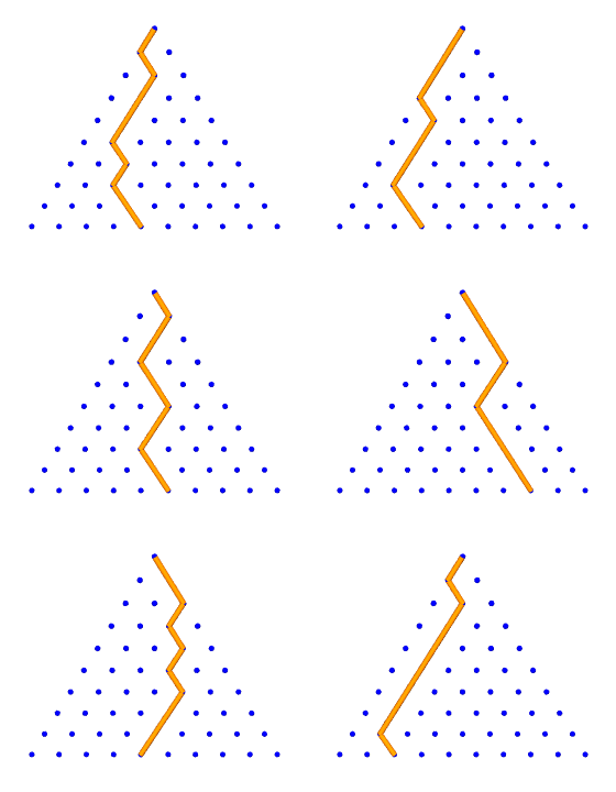
Pascal's Triangle relates to the Japanese pin-ball game, Pachinko, wherein user-fired balls fall through a lattice of pins, by chance dropping into special cups, in which case points are awarded.

The lattice is triangular, like Pascal's Triangle, meaning a ball will fall either left or right to the next row, where it will encounter another pin, fall left or right again and so on.


If we envision a simplified Pachinko board wherein all balls begin their fall at the same apex, and proceed down the lattice, falling either leftward or rightward at random, then, over time, we will find the majority of balls exit towards the center of the pattern.

The reason for this is most random paths of leftward and rightward moves contain approximately the same number of lefts as rights, meaning an average ball does not stray very far from the center. Less frequently, lefts will greatly outnumber rights or vice versa.

image


We can associate each bottom pin with the "number of lefts" (or rights) it would take to reach it. The leftward and rightward extremes at each row are attained only if a ball always falls in the same direction -- an increasingly unlikely outcome, the more rows we allow it to fall.

We can run our trials in Python to get a sense of the relative frequencies involved. The random module, one of the standard extensions to the language, includes a choice function, which takes a list as input and returns a random selection from the list as output.

>>> import random
>>> mylist = ['Pig', 'Dog', 'Cat', 'Camel', 'Star Fish', 'Zebra']
>>> random.choice(mylist)
'Star Fish'
>>> random.choice(mylist)
'Camel'
>>> random.choice(range(5))
2
>>> random.choice(range(5))
0

Consider a cubical die (as in "one die, two dice"): we might model it with a list of 6 possible, equally likely, outcomes: [1,2,3,4,5,6]. Of course if the die is "loaded" then the outcomes are not equally likely.

In some games, 8 or even 20-sided dice are used, so lets have a Python class called Die, which is flexible about how many faces (outcomes) it has. We will then cast our die one or more times, to get our randomized results.

>>> import rand
 >>> ofuzzy = rand.Die()
 >>> ofuzzy.faces = 2 
 >>> ofuzzy.cast(4)
 [1, 1, 1, 0]
 >>> ofuzzy.faces=12
 >>> ofuzzy.cast(10)
 [7, 7, 5, 0, 2, 2, 9, 2, 8, 10]

class Die:

    faces  = 2  # number of faces
    lowest = 0  # lowest number face
    
    def cast(self,n):
        # return a list with die rolled n times
        trials = []
        options = range(self.lowest,self.faces+self.lowest)
        for i in range(n):
            trials.append(random.choice(options))
        return trials

Returning to our model of falling Pachinko balls, lets think of left as 0 and right as 1. By casting a two-sided die object N times, and adding all the 1's, we get the number of rightward moves down a path of N falls.

We can tally our trials by incrementing a counter for each exit pin by one, each time a ball reaches the last row. Each pin is uniquely identified by the "number of rights" it takes to reach it. In other words, the leftward and rightward moves taken by each ball during its downward trajectory may come in any order, but it's their relative number which uniquely determines the exit pin.

>>> import rand
>>> odie = rand.Die()      # two faces by default, 0 & 1 as possibilities
>>> trials = odie.cast(10) # cast the die 10 times, storing to trials 
>>> trials                 # show list
[0, 0, 0, 0, 0, 0, 0, 0, 0, 1]
>>> trials.count(1)        # count how many 1s (i.e. how many "rights")
1
>>> trials = odie.cast(10) # cast again, for another list of 10 outcomes
>>> trials                 # show list
[1, 1, 1, 1, 0, 1, 1, 1, 1, 1]
>>> trials.count(1)        # count how many 1s (remember, it's random)
9

How many trials shall we run? The numerical entries in Pascal's Triangle (or Tetrahedron) give a count of the number of pathways to that pin (vertex, sphere). In a random system, the number of encounters with a pin should be directly proportional to the number of pathways leading to it. If "all roads lead to Rome", then many travelers should encounter Rome, even if they wander aimlessly.

So let's add up all the entries in row N of Pascal's Triangle, thinking "this is the total number of balls that exited through this bottom row", and then compare bottom row entries with the exit tallies generated by our random trials. Our random trials are provided by the rand.binomial function.

>>> import rand
>>> import series
>>> rand.binomial(10) # 11 numbers because compared with Pascal's Triangle
[0, 12, 48, 124, 202, 245, 214, 130, 42, 5, 2]
>>> map(int,series.prow(10)) # rows start from 0, row 10 has 11 entries
[1, 10, 45, 120, 210, 252, 210, 120, 45, 10, 1]
>>> rand.binomial(12) # falling through to row 12 (of 13 spheres)
[2, 9, 63, 220, 510, 757, 946, 812, 479, 220, 65, 11, 2]
>>> map(int,series.prow(12)) # Pascal's Triangle entries close to same
[1, 12, 66, 220, 495, 792, 924, 792, 495, 220, 66, 12, 1]

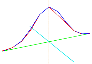
At right we compare graphs generated by series.prow(10), which generates row 10 of Pascal's Triangle, and rand.binomial(10), which runs random trials through the same number of rows. The graphs show up and red and blue respectively, and are clearly giving similar results.

>>> import bellcurve, povray
>>> import functions
>>> g =Povray("gaussian.pov")
>>> bellcurve.gauss(10,g)
>>> myfile.cylcolor="Red"
>>> bellcurve.gauss(10,g,2)
>>> functions.xyzaxes(g,4)
>>> g.close()

Source code for bellcurve.gauss is included in Section 2.

image

Gaussian Distributions: Pascal's Triangle, Random Trials


The path of each Pachinko ball is an example of what we call a random walk in a matrix, or lattice. In addition to falling balls, encourage your students to use the turtle metaphor -- perhaps a swimming sea turtle.

Of course a "turtle" is also a graphical cursor, and a hallmark of the Logo language. Students entering your course with some background in Logo will find this reference to a turtle positively reinforcing.

We will be defining a Turtle object in Python below, and endowing it with the power to leave a graphical trail in Povray, as per our characteristic "dynamic duo" strategy. At each "turn to play" our turtle must select from the range of freedoms available to it.

In the case of Pascal's Triangle, or Pascal's Tetrahedron, the turtle has two or three degrees of freedom respectively, always in the "downward" direction (unless we want define a more gravity-free environment, leading to more freedoms).


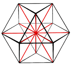
Other freedoms, each characteristic of a different lattice, might include the mutually perpendicular i,j vectors in the XY plane, or the i,j,k vectors in XYZ. We could also define the vectors from the center to the four corners of a regular tetrahedron as freedoms, or from the center to the 12 corners of a cuboctahedron.

These latter options are more characteristic of the non-rectilinear sphere packing lattices. Our Python Turtle class accepts a list of vectors when objects based on this class are instantiated. These become the freedoms, and their number determine how many sides the "internal die object" is defined to have.

image
12 degrees of freedom


The code below shows a lot of the essential guts of our Turtle class.

from coords import Vector
import rand
import shapes

phi = (1 + 5**0.5)/2.0
root2 = 2.0**0.5

class Turtle:

    def __init__(self,freedoms,drwfile):
        self.freedoms = freedoms  # list of vectors
        self.drawfile = drwfile   # Povray object
        self.location = Vector((0,0,0)) # turtle's current location
        self.color = 'Red'              # turtle's current color
        self.trail = []           # records sequence of directional hops
        self.ofuzzy = rand.Die()  # a die object for randomizing hops
        self.penstate = 1         # pen is up or down        

    def randomwalk(self, steps=1):
        # hop randomly for some steps
        self.ofuzzy.faces = len(self.freedoms)
        for x in range(steps):
            dir = self.ofuzzy.cast(1)
            self.move(dir[0],1)

    def move(self, direction, steps=1):
        # hop in freedoms[direction] x steps
        for x in range(steps):
           newloc = self.location + self.freedoms[direction]
           self.trail.append([direction,steps])
           if self.penstate == 1:               
               self.drawpath(self.location,newloc)
           self.location = newloc

Here we have an example of "object composition": the turtle objects have die objects inside of them.

Our Turtle also accepts manually entered instructions: the user types which direction to move in by number, with N freedoms automatically designated by 0 through (N-1) -- a convention students might wish to change to 1 through N by reprogramming. Encourage your students to experiment and explore by making changes in the code.

    def manual(self):
        print "Manual mode (-1 to quit):"        
        while 1:            
           dir = input("?: ")
           if dir == -1: break
           elif not dir in range(len(self.freedoms)):
             print "Invalid direction: range 0-"+str(len(self.freedoms)-1)
           else: self.move(dir,1)

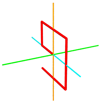
Below we interactively define and operate a manual turtle in the YZ plane, with the resulting mywalk.pov shown at right.


>>> from povray import Povray
>>> from coords import Vector
>>> from turtles import Turtle
>>> import functions
>>> mywalk = Povray("mywalk.pov")
>>> z = Vector((0,0,1))
>>> y = Vector((0,1,0))
>>> freedoms = [z,-z,y,-y]
>>> oturt=Turtle(freedoms,mywalk)
>>> functions.xyzaxes(mywalk,2)
>>> mywalk.cylradius = 0.04
>>> mywalk.cylcolor = "Magenta"
>>> oturt.manual()
Manual mode (-1 to quit):
?: 0
?: 2
?: 1
?: 1
?: 3
?: 3
?: 0
?: 0
?: -1
>>> mywalk.close()

image
mywalk.pov

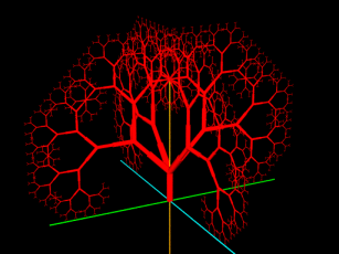
Another species of turtle is able to trace out much more complicated paths based on only a few lines in a formal symbolic code known as an L-system.

The L-system turtle or Lturtle comes with an instruction set of about 30 single-letter commands -- some of which cause the turtle to reorient itself at random. Substitution rules combine these commands into longer and longer strings, spelling out every twist and turn in a complicated, yet repetitious, journey.

The fractal tree at right was produced using Python + Povray from the coded L-system instructions below.

# An L-System file
9         # recursive depth
45        # turn angle
10        # thickness as a %
+(90)c(2)AB         # Axiom
A = [F[+FCA][-FCA]] # Rule
B = [F[^FCB][&FCB]] # Rule
C = '(0.7071)       # Rule
@
image

This curriculum was among the first to take significant advantage of R. Buckminster Fuller's philosophical explorations to advance its goals. Oregon Curriculum Network goals include:
  • moving beyond flatland using computer technology
  • presenting polyhedra as objects when teaching OOP
  • developing a capacity for "mental geometry" not just "mental arithmetic"
  • encouraging more comprehensive modes of thinking about whole systems

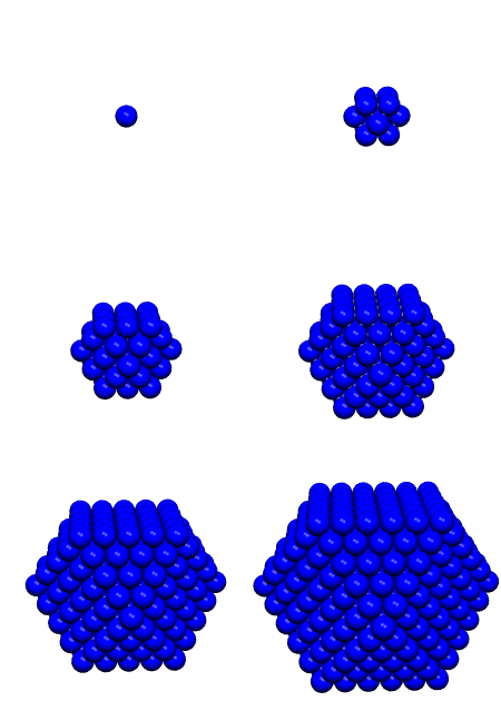
Fuller's approach centers around polyhedra organized in a concentric hierarchy within a uniform sphere packing -- the same cuboctahedrally-conformed sphere packing studied by Johannes Kepler (1571-1630), William Barlow (1845-1934) and many others.

Within this hierarchy, the tetrahedron, formed by four intertangent unit-radius spheres, is assigned a volume of unity, and thereby becomes the standard "measuring cup" to which all other volumes are referenced. The hierarchy includes many structural relationships familiar to geometers, including the jitterbug transformation, mentioned in earlier sections 1 and 2.

image
cuboctahedrally-conformed
uniform sphere packing

This unit-volume tetrahedron convention has some significant, streamlining advantages and is well worth sharing with your students.
>>> tetra = shapes.Tetra() # edge=sphere diameter
>>> octa = shapes.Octa()   # same edges
>>> cubocta = shapes.Cubocta() # same edges
>>> tetra.volume()   # tetra has unit volume
1.0
>>> octa.volume()    # has a whole number volume
4.0
>>> cubocta.volume() # ditto
20.0
>>> shapes.Icosa().volume()
18.5122958682        # ... but not the icosa
image
concentric hierarchy around a single lattice sphere

Our approach is also backward-compatible with more conventional ones. By analogy, if you learn Python, a relatively new computer language, this does not entail your unlearning BASIC or C.

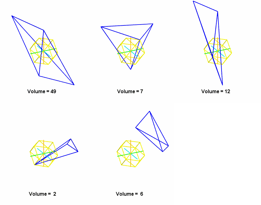
One interesting consequence of using this alternative measuring cup is that any tetrahedron with lattice point vertices will have a whole number volume. We can test this claim programmatically in Python, using our new Turtle objects. Robert Gray has also provided a formal, deductive proof.

Set four Turtle objects at the origin and define their degrees of freedom to be the 12 vectors to neighboring sphere centers in the lattice.

Allow all four turtles to wander randomly for N hops -- they will usually end up further away from one another, although of course it's possible for two turtles to land on the same vertex (meaning we would not get a tetrahedron), or for all four to end up on the same plane (likewise meaning no volume).

In non-degenerate cases (where tetrahedra are actually formed -- though rarely regular ones), we compute their volumes using the six edge lengths as inputs.

The result is always a whole number, remembering that a 1x1x1 tetrahedron, with six sphere-diameter edges, is unity by definition.

image


Here's some code for generating random tetrahedra using four turtles free to wander in a sphere packing lattice:
def randtet(canvas):
    
    # 12 degrees of freedom (to corners of cubocta)
    freedoms = turtles.ivmrays()

    v = []            # list to receive vertices
    tlist = [0,0,0,0] # list to receive turtles

    # initialize four turtles
    for i in range(4):
       tlist[i] = turtles.Turtle(freedoms,canvas)
       tlist[i].penup()  # don't show walks

    # let each take six steps
    for t in tlist:
       t.randomwalk(6)
       v.append(t.location) # append a vector
    
    # use the four randomly derived vertices
    # to define a tetrahedron    
    otetra = shapes.Tetra(v[0],v[1],v[2],v[3])

   # get the volume    
    vol = otetra.volume()

    # discard volumes < 1
    if vol<1: rtnval = "Degenerate"
    else:
       rtnval = vol
       if canvas:
          # draw the tetrahedron  
          otetra.drawself(canvas)

    # print tetrahedron's volume
    print vol
    
    # return tetrahedron object
    return otetra

Usage:

>>> myfile = povray.Povray("randomtet.pov")
>>> for i in range(6): rand.randtet(myfile) # draws, prints volumes

40.0
4.0
13.0
9.0
28.0
6.0
>>> myfile.close()

Another interesting fact is that the respective perpendiculars to the four faces of any tetrahedron, with lengths proportional to facial areas, cancel out. The sumnormals function accepts a random tetrahedron as input and performs the necessary cross-product computations -- the result should always be zero.

>>> mytet = rand.randtet()
18.0
>>> rand.sumnormals(mytet)
0.0

This essay was designed to suggest a number of branch points to connected topics, some more explored than others. You of course have a lot of disgression in how you might want to fit these threads into a curriculum of your own.

From this discussion of random walks constrained by degrees of freedom, you might want to explore the topic of quadrays, a game with non-hyperdimensional 4-tuple vectors based on the 4 freedoms of the tetrahedron (see section 2). Following this fork in the road will bring you back to many points already visited in this essay, plus may encourage your students learn to think more generically about data structures and operations.

Or you might want to jump to the topic of spherical coordinates at this juncture, for many of the same reasons i.e. to show how the same position information might be encoded in alternative formats or data structures.

You'll find the coords.py module includes subclasses of the Vector class, Svector and Qvector, which accept arguments in either spherical or quadray formats respectively. In all other respects, these additional subclasses of vector behave just like their parent class and may be combined with one another in vector operations.

>>> import shapes
>>> from coords import *
>>> v1 = Qvector((1,0,0,0)) # vectors to 4 corners of a reg tetrahedron
>>> v2 = Qvector((0,1,0,0))
>>> v3 = Qvector((0,0,1,0))
>>> v4 = Qvector((0,0,0,1))
>>> otetra = shapes.Tetra(v1,v2,v3,v4)  # create the shape
>>> otetra.volume()                     # get its volume
1.0
>>> v1.angle(v2)    # central angle of a regular tetrahedron
109.47122
>>> v4.spherical()  # r = quadray length relative to sphere diameter
(0.612372435696, 125.264389683, -45.0)
>>> v3 = -Svector(v4.spherical()) # define Svector pointing oppositely
>>> v3.angle(v4)    # confirm angle between them is 180 degrees
180.0
>>> v5=v3+v4        # add Svector and Qvector (oppositely oriented)
>>> v5.xyz          # check xyz coordinates of resulting vector
(0.0, -5.55111512313e-017, 0.0)

For further reading:


oregon.gif - 8.3 K
Home Page