Jiving In J:
Towards Enlivening Our K-12
Mathematics Curricula
Mathematics Curricula
by Kirby Urner
Oregon Curriculum Network
First posted: July 13, 2002
Last updated: Sept 14, 2002
Table of Contents:
- The Live Languages Movement
- The More the Merrier
- Jiving in J
- Using J to Explore Basic Number Concepts
- Linking to Abstract Algebra
- Deepening the Connections Over Time
- Speculation
- Notes
- For Further Reading
First draft posted to math-teach
1. The Live Languages Movement
As long time subscribers to math-teach at the Math Forum well know, I frequently push computer languages as a way to add spice and relevance to math classes.(1)
Non-executable symbolic notations just sit there, so we might reasonably call them dead languages, in the sense of non-vital, but perhaps in the more usual sense as well: headed the way of Latin.
It might be argued that mathematical notation (to be referred to as MN) is adequate as it is, and could not benefit from the infusion of ideas from programming languages. However, MN suffers an important defect: it is not executable on a computer, and cannot be used for rapid and accurate exploration of mathematical notions. (Iverson, 2)
To have your writing surface come alive with self-executing symbols is to enter the world of live languages, of which we have a growing number.
Calculators were the cutting edge of the live language movement, cheaper and more portable than computers, ever more programmable, and in many ways closer to the math, with primitives for doing trig, standard deviation and, more recently, plotting curves.
But computers have come a long way in terms of the price/performance ratio and the live language movement is entering a new phase with an even greater variety of pedagogical opportunities.
I've been making the case for Python as a first language, to be learned in conjunction with math topics, given its clean syntax and intuitive implementation of time-tested concepts.
Python is cosmopolitan, in that it gets ideas from many more specialized, more academic languages (e.g. Icon, Haskell). This helps makes it another "grand central" node in our curriculum i.e. a node characterized by its more-than-usual number of connections to other nodes.(Urner, 3)
However, I also consistently make the case that no serious student should stop at one language, which is to artificially deprive oneself of the vast riches our cultures have to offer.
In an effort to practice what I preach, I've been recently delving into the J language, thanks to a tip from Fraser Jackson, who'd been perusing some of my web-based evangelism on behalf of Python (Urner, 4). In particular, he'd been looking at a paper where I compare Python to a first love (the first language I encountered at Princeton): APL (A Programming Language).
J is a next generation APL, again by APL's architect Ken Iverson, in collaboration with Roger Hui. Unlike APL, which required a specialized keyboard with greek-looking symbols, J uses the regular ASCII character set. However, like APL, it is designed to be an executable math notation.
Like all languages suitable for on-the-fly investigations and explorations, J is interactive: type an expression, get an immediate evaluation. Scheme, ISETL, Logo and Python all feature this immediate feedback cycle, a shell mode. Java and C/C++ do not.
J is very math-focused. Iverson has written a companion to Concrete Mathematics, a classic text book for computer science majors, but relevant to anyone (it reminds me of Conway's and Guy's The Book of Numbers, another classic, for which Iverson is doing another companion guide).
Of even more relevance to this list, J comes with a lab closely synched with Saxon Math. Quoting directly from the docs:
Lab Section A. Purpose
This program is designed to accompany the text "MATH 87", by Stephen Hake and John Saxon, Saxon Publishers, Norman, Oklahoma, 1997. It follows the text closely, and uses the programming language J to illustrate and illuminate the topics (5)
Certainly the next time I chat with a parent at some homeschooler conference (I've been an invited speaker to such), and said parent confesses to using Saxon Math at home, I'll say "that's great -- have you checked into using it in complement with J?". A conversation might ensue from there. Certainly we have plenty of opportunities here to supplement Saxon, or other math learning texts, with additional J-based materials, and make them freely available to students over the internet.
Just to delve into J a bit, let's quote from the console for awhile and see what makes it fun.
Right off the bat, you find some high level verbs (as they're called), like q: which outputs the prime factors of a number (up to some large limit).
   q: 200192     NB.  get the prime factors of 200192
2 2 2 2 2 2 2 2 2 17 23
   q: 883821     NB.  <-- means 'comment' (not evaluated)
3 23 12809
The insert operator modifies a verb (is an adverb) to make it insert between the nouns that follow. For example, */ 3 2 1 means 3 * 2 * 1 i.e. outputs 6. So the */q: of a positive integer should give back the integer itself:
   */q: 43889    NB. putting humpty dumpty back together
43889
   */q: 12882938
12882938
Suppose we just want the unique prime factors of a number. The ~. verb picks out unique elements:
   ~.q: 200192
2 17 23
We can assign this dual-action to a name of our own choosing, provided we look at the pattern. It's the application of two monadic functions: q: spits out an array and ~. grabs the unique elements.
If we name each verb separately...
   factors =: q:
   unique  =: ~.
then what we want is unique(factors(n)). f(g(x)) is simply f g x in J, provided both f and g are monadic (i.e. accept one element on the right).
   unique factors 200192
2 17 23
Now suppose we want a single verb that captures the sense of (f(g(x)) -- except we're not providing any argument (no x). This requires the use of a conjunction, @, which, in the case of monadic functions, simply glues them together.
   upfs =: unique @ factors  NB. new verb w/ composition

   upfs 200192
2 17 23
To further clarify the use of @, suppose we wanted to double a number, square it, then take its reciprocal. J has primitive verbs for each of these operations: +: *: and % respectively. If we're ready to apply these to a noun, we could just go:
   % *: +: 10
0.0025
This train of verbs makes sense as long as we have a noun at the end, permitting immediate evaluation. J executes right to left, unless instructed to do otherwise by parentheses, so this is actually the same as writing
   % (*: (+: 10))            NB. double, then square, then reciprocate
0.0025
However, if what we want is a new verb, containing the sense of the whole operation, but without a noun, then we need @ to glue our verbs together. @ is called a conjunction, meaning it takes two verbs as arguments (adverbs take only one verb, / being an adverb we've used previously, as in */ q:).
So we could compose our verbs with @ as follows:
   newverb =: % @ *: @ +:    NB. f(g(r(x)))
   newverb 10
0.0025
   %(10+10)^2                NB. putting it another way
0.0025
And in this case, since % *: and +: all naturally apply to arrays, we can apply our newverb to a whole sequence at once:
   newverb 10 11 12
0.0025 0.00206612 0.00173611
4. Using J to Explore Basic Number Concepts
In the traditional K-12 curriculum, we introduce primes versus composite numbers in connection with factoring. We give some attention to the GCD and LCM, perhaps in connection with rational numbers i.e. fractions. In order to simplify or reduce a fraction, you in effect divide out any greatest divisor in common between the numerator and denominator.
J has the dyadic verb +. which means GCD when placed between integers.
   12 +. 5
1
   27 +. 3
3
Since 27 and 3 have the common factor of 3, the fraction 3/27 simplifies to 1/9. Unlike many computer languages, J has a built in rational number type, signified as NrD where N is the numerator, D the denominator. In creating the fraction 3/27, we see the reduction to lowest terms is automatic:
   3r27      NB. J has a native rational type (complex too)
1r9
However, once these basics are introduced, the traditional K-12 curriculum is usually in a big hurry to escape the pure integers, by way of fractions, and on to reals, and so it doesn't allow any more time with simple number theory concepts, which I think is poor design.
The concepts of GCD and prime number would anchor better if we did more to nail them down, meaning linked them to other nodes in the curriculum more tightly.
For example, if two integers have no factors in common other than 1, we say they're relatively prime, or coprime.
If you take any positive integer n and look at all the integers less than or equal to it, down to 1, they break into two categories:
(a) those which have factors in common with n, and
(b) those which do not.
Among those with factors in common, you have two subcategories:
(a.1) those which divide into n (the divisors, including n), and
(a.2) those which merely share factors.
For example, 27 has a divisor of 3, but 6, while it shares 3 as a factor, doesn't divide into 27 without remainder. 8, on the other hand, doesn't even share factors with 27, meaning, of course, it can't divide it either (or it would itself be a factor).
Using J's primitives, we can find all positives <= n with no factors in common (the so-called "totatives of n" -- the number of which is the "totient of n"), by using the dyadic GCD verb (takes two arguments).
Let's put n on one side, and an array 1...n on the other (in this case, either order would work). J is especially powerful because, like APL, it's about as easy to operate with arrays (including multi-dimensional) as with scalars.
   1 2 3 4 5 6 7 8 9 10 11 12 +. 12
1 2 3 4 1 6 1 4 3 2 1 12
or
   12 +. 1 2 3 4 5 6 7 8 9 10 11 12
1 2 3 4 1 6 1 4 3 2 1 12
Wherever a 1 occurs in the output, we've got a coprime to 12. We can isolate these by testing for "equal to 1":
   1 2 3 4 1 6 1 4 3 2 1 12 = 1
1 0 0 0 1 0 1 0 0 0 1 0
Now if we could use this pattern of 1s and 0s to select from the original list (1-12), we'd have the totatives of 12 in an array. J has the verb we need (#):
   1 0 0 0 1 0 1 0 0 0 1 0 # 1 2 3 4 5 6 7 8 9 10 11 12
1 5 7 11
Likewise, if we flip the 1s to 0s and 0s to 1s, we'll get those numbers with factors in common.
   1 2 3 4 1 6 1 4 3 2 1 12 > 1       NB. selecting if > 1
0 1 1 1 0 1 0 1 1 1 0 1
Selecting from the original list:
   0 1 1 1 0 1 0 1 1 1 0 1 # 1 2 3 4 5 6 7 8 9 10 11 12
2 3 4 6 8 9 10 12
Of this latter set, some are actual divisors of 12, meaning their factor in common is the number itself. Equivalently, they divide into 12 with no remainder. To get the remainder, we can apply dyadic | (as a monad, this same verb returns the magnitude or absolute value of its argument):
   2 3 4 6 8 9 10 12 | 12             NB. divisors generate 0 remainder
0 0 0 0 4 3 2 0
Putting all this together, we have strategies for outputting the totatives (i.e. positives <= N and coprime to N), as well as the non-totatives (positives <= N but with factors in common) and the divisors (positives <= N which divide into N with no remainder).
Let's write tots, ntots, divs as explicit programs.(Note, 6) They're all monads, meaning they take a single argument, referred to as y. in the body of the program. Monads are 'type 3' constructs (of four types in all), and we can define them like this:
   tots =: 3 : 0          NB. means 'define a monad as follows'
pos =. >: i.y.            NB. non zero positives <= y.
sel =. 1 = pos +. y.      NB. get string of 1s and 0s
sel # pos                 NB. return selection (paren ends program)
)
Testing:
   tots 12
1 5 7 11
   tots 28
1 3 5 9 11 13 15 17 19 23 25 27
We see a couple new verbs in tots (like when learning a human language, we gradually add to the vocabulary). i. creates an array of integers from 0 to n-1 given noun n, e.g. i.12 returns 0 1 2 3 4 5 6 7 8 9 10 11. However, we'd like 1 through 12, so we use the >: verb (increment) to bump every element up by one.(Note, 7)
The results get assigned to pos, which then goes against 12 using the GCD verb.(Note, 8) The output is compared to 1 using = and gives an array of 1s and 0s as discussed above, which is then used to pick out just the totatives.
The non-totatives are extracted almost the same way:
   ntots =: 3 : 0
pos =. >: i.y.            NB. non zero positives < or equal to y.
sel =. 1 < pos +. y.      NB. get string of 1s and 0s
sel # pos                 NB. return selection
)

   ntots 12
2 3 4 6 8 9 10 12
   ntots 15
3 5 6 9 10 12 15
The only difference is an equal sign was replaced with a less than sign, which exchanges 1s and 0s from the previous output (which is interimly stored in sel).
Now we'd like to spit out the true divisors of n. We might as well start with the non-totients, with the further restriction that no remainder is left when dividing a candidate into the target.
   divs =: 3 : 0
candidates =. ntots y.
sel =. 0 = candidates | y.        NB. test for 'no remainder'
sel # candidates
)


   divs 12
2 3 4 6 12
   divs 27
3 9 27
   divs 100
2 4 5 10 20 25 50 100
The number of totatives of n is called the totient of n, which we may define simply as the length of the list returned by tots.
totient =: 3 : '# tots y.' NB. note shortened syntax for one-liners
or even just:
totient =: # @ tots NB. composing # with tots(n) = #(tots(n))
Testing:
   totient 100
40
   totient 12
4
The totient concept has a lot of relevance in number theory, and we could and should show some of this relevance -- even to 7th or 8th graders when in preview mode.
For example, Euler's theorem states that if you take some base integer with no factors in common with n, and raise that base to the totient(n) power, and then divide by n, the remainder is always 1.
The proof isn't difficult, but it can wait. The important thing at the introductory level is (a) to get the meaning of a theorem and (b) to test it, play with it, by implementing it in an executable form.
   euler =: 4 : 0       NB. euler is a dyad, with base on the left
y. | x. ^ totient y.    NB. left argument is x. and right is y.
)


   2 euler 19           NB. i.e. 19 | 2^(totient 19) returns remainder 1
1
   2 euler 35
1
   3 euler 28           NB. 3 and 28 have no factors in common
1
This version of an "Euler's Theorem tester" will fail when the powers get high enough to push the result into a floating point number, in advance of dividing by the right argument.
   3 +. 205             NB.  GCD(3, 205) = 1, so we expect 3 euler 205 = 1
1
   3 euler 205          NB.  But it isn't
0
   totient 205          NB.  to what power was our base of 3 raised?
160
   3^160                NB.  a floating point! messes up the last step
2.18475e76
This limitation may be overcome using an extended precision symbol x, which becomes part of a number's format. Just as 3r4 is the format of a rational number, and 3j4 the format of a complex number, so is 2x the format of an extended precision integer of value 2. An extended precision integer raised to power invokes different (slower, precision-preserving) algorithms in the J interpreter.
   base=:2              NB.  base is assigned ordinary integer 2
   base                 NB.  note how it looks when given as output
2

   base^200             NB.  gives a large floating point answer
1.60694e60

   base^2000            NB.  i.e. infinity; decimal format limit exceeded
_
   base =: 2x           NB.  now base is extended precision 2
   base                 NB.  outwardly, it looks just like ordinary 2...
2

   base^200             NB.  ...but look how we keep full precision
1606938044258990275541962092341162602522202993782792835301376

   base^2000            NB.  the console gives up, ends with '...'
1148130695274254524232833201177681984022317702088695200477642
7368257662613923703138566594863165062699184459646389874627734
4711896086305533142593135616665318539129989145312280000688779
1482400448714289269900634862447816154636463883639473170260404
663539709049...
To get around the limitations of ordinary console output, when it comes to these super large extended precision numbers, we need to draw on one of J's pre-scripted utility functions, xfmt.
   load 'format'        NB. load pre-defined verbs from a file

   75 xfmt base^2000    NB. a utility, left argument sets width to 75
  114 81306 95274 25452 42328 33201 17768 19840 22317 70208 86952 00477
64273 68257 66261 39237 03138 56659 48631 65062 69918 44596 46389 87462
77344 71189 60863 05533 14259 31356 16665 31853 91299 89145 31228 00006
88779 14824 00448 71428 92699 00634 86244 78161 54636 46388 36394 73170
26040 46635 39709 04996 55816 23988 08944 62960 56233 11649 53616 42219
70332 68134 41689 08984 45850 56023 79484 80791 40589 00934 77650 04290
02716 70662 58305 22008 13223 62812 91761 26788 33172 06598 99539 64181
27021 77985 84040 42159 85318 32515 40889 43390 20919 20554 95778 35896
72039 16008 19572 16630 58275 53804 25583 72601 55283 48786 41943 20545
08915 27578 38826 25175 43552 88008 22842 77081 79654 53762 18485 11490
29376

   euler =: 4 : 0       NB.  new definition
base =. x:x.            NB.  verb x: casts x. to extended precision
y. | base ^ totient y.  NB.  same as before
)

   3 euler 205          NB.  ...and now this works (but see below)
1
A deeper problem here is, even if we add extended precision, our strategy of raising a base to a large power, only to divide to get a remainder, is very inefficient. If you try 3 euler 200005 with the above version, you will get the right answer, but the computer will start taking awhile, as 3^totient(200005) is a rather big number to find (even though the interpreter knows some short cuts).
A much better approach is to apply a "divide as you go" strategy. That keeps the computation from interimly skyrocketing through the roof on an exponential trajectory.
This optimization is accomplished internally by the interpreter, if triggered by conjoining exponentiation to the residue operator with @ as shown below. This is starting to be a more advanced level of J than we would probably need at first, but it's good to know that the language designers have given us these streamlining powers.
   euler =: 4 : 'x. (y.&| @ ^) totient y.'

   3 euler 200005      NB.  Doesn't take much time at all
1
5. Linking to Abstract Algebra
The totatives come into abstract algebra in that if you multiply totatives of n modulo n, you always get another totative, meaning we have closure. For example, since:
   tots 12
1 5 7 11
Any products of these totatives, divided by 12, will have a remainder that's likewise one of these totatives.
   12 | 5*7
11
   12 | 11*5
7
We can generate a multiplication table after defining the verb x12, which multiplies and gets the remainder after dividing by 12.
   x12 =: 12&| @ *

   x12 table tots 12
+--+-----------+
|  | 1  5  7 11|
+--+-----------+
| 1| 1  5  7 11|
| 5| 5  1 11  7|
| 7| 7 11  1  5|
|11|11  7  5  1|
+--+-----------+
The & binds the 12 to the dyadic |, making 12&| a monad, which in turn applies to the output of dyadic * (multiplication).
The @ conjunction is used pretty much as before, to compose the 12&| monad with the * dyad. When the function on the left is dyadic, the pattern changes: f(g(x)) means x f g(x) in that case, called a hook pattern (there's also a fork pattern).
Note also that every totative of 12 has an inverse, meaning a paired element such that the product is 1. 1 is that element which has no effect when used with our x12 -- which is why it's called an identity element. 1, 5 and 7 are their own inverses (reading along the diagonal of the table).
Multiplication with x12 is also associative. Letting the generic multiplier * stand in for x12, we might write: t1 * (t2 * t3) is always the same as (t1 * t2) * t3, which in turn means that t1 * t2 * t3 is unambiguous even without parentheses.
These four properties:
- closure
- the presence of an identity element (neutral element)
- every element has an inverse
- associativity
are necessary and sufficient to call this set of elements a group with respect to the x12 operation (which is a kind of multiplication).(Note, 9)
Given multiplication modulo M is also commutative, this is a commutative group as well (also known as an Abelian group).
But we don't have a field here. Even if we include the additive identity 0, we still don't have closure under addition modulo M, defined as follows:
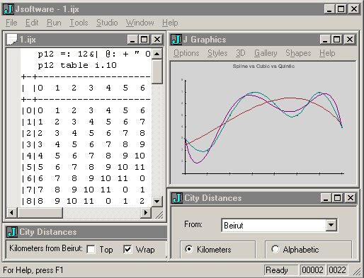
p12 =: 12&| @ +
The built-in table utility, defined with more primitive verbs, adverbs and conjunctions, will do a Cartesian cross product using our choice of dyadic verb, and produce the result in tabular format:
   p12 table 0,tots 12      NB. comma joins 0 output of tots 12
+--+--------------+
|  | 0  1  5  7 11|
+--+--------------+
| 0| 0  1  5  7 11|
| 1| 1  2  6  8 12|
| 5| 5  6 10 12 16|
| 7| 7  8 12 14 18|
|11|11 12 16 18 22|
+--+--------------+
Some of the elements in the table do not appear in the header or leftmost column, meaning we are not seeing closure.
However, if instead of composite number 12, we take any prime number Z as our modulus, then we get commutativity, closure and associativity under addition (abelian group), plus the same properties under multiplication (another abelian group). Finally, we have the distributive property linking the two operations i.e. a*(b+c) = a*b + a*c.
And these are all the properties you need to achieve fieldhood (abelian grouphood for both + and *, along with distributivity to link them).
J will spit out the nth prime number Z given the p: verb.
   p: 6                      NB. get a modulus
17
   tots 17                   NB. list its totatives
1 2 3 4 5 6 7 8 9 10 11 12 13 14 15 16


   p17 =: 17&| @ +
   x17 =: 17&| @ *

   p17 table 0,tots 17       NB. prefixing 0 as an element
+--+--------------------------------------------------+
|  | 0  1  2  3  4  5  6  7  8  9 10 11 12 13 14 15 16|
+--+--------------------------------------------------+
| 0| 0  1  2  3  4  5  6  7  8  9 10 11 12 13 14 15 16|
| 1| 1  2  3  4  5  6  7  8  9 10 11 12 13 14 15 16  0|
| 2| 2  3  4  5  6  7  8  9 10 11 12 13 14 15 16  0  1|
| 3| 3  4  5  6  7  8  9 10 11 12 13 14 15 16  0  1  2|
| 4| 4  5  6  7  8  9 10 11 12 13 14 15 16  0  1  2  3|
| 5| 5  6  7  8  9 10 11 12 13 14 15 16  0  1  2  3  4|
| 6| 6  7  8  9 10 11 12 13 14 15 16  0  1  2  3  4  5|
| 7| 7  8  9 10 11 12 13 14 15 16  0  1  2  3  4  5  6|
| 8| 8  9 10 11 12 13 14 15 16  0  1  2  3  4  5  6  7|
| 9| 9 10 11 12 13 14 15 16  0  1  2  3  4  5  6  7  8|
|10|10 11 12 13 14 15 16  0  1  2  3  4  5  6  7  8  9|
|11|11 12 13 14 15 16  0  1  2  3  4  5  6  7  8  9 10|
|12|12 13 14 15 16  0  1  2  3  4  5  6  7  8  9 10 11|
|13|13 14 15 16  0  1  2  3  4  5  6  7  8  9 10 11 12|
|14|14 15 16  0  1  2  3  4  5  6  7  8  9 10 11 12 13|
|15|15 16  0  1  2  3  4  5  6  7  8  9 10 11 12 13 14|
|16|16  0  1  2  3  4  5  6  7  8  9 10 11 12 13 14 15|
+--+--------------------------------------------------+

   x17 table tots 17         NB. not including 0
+--+-----------------------------------------------+
|  | 1  2  3  4  5  6  7  8  9 10 11 12 13 14 15 16|
+--+-----------------------------------------------+
| 1| 1  2  3  4  5  6  7  8  9 10 11 12 13 14 15 16|
| 2| 2  4  6  8 10 12 14 16  1  3  5  7  9 11 13 15|
| 3| 3  6  9 12 15  1  4  7 10 13 16  2  5  8 11 14|
| 4| 4  8 12 16  3  7 11 15  2  6 10 14  1  5  9 13|
| 5| 5 10 15  3  8 13  1  6 11 16  4  9 14  2  7 12|
| 6| 6 12  1  7 13  2  8 14  3  9 15  4 10 16  5 11|
| 7| 7 14  4 11  1  8 15  5 12  2  9 16  6 13  3 10|
| 8| 8 16  7 15  6 14  5 13  4 12  3 11  2 10  1  9|
| 9| 9  1 10  2 11  3 12  4 13  5 14  6 15  7 16  8|
|10|10  3 13  6 16  9  2 12  5 15  8  1 11  4 14  7|
|11|11  5 16 10  4 15  9  3 14  8  2 13  7  1 12  6|
|12|12  7  2 14  9  4 16 11  6  1 13  8  3 15 10  5|
|13|13  9  5  1 14 10  6  2 15 11  7  3 16 12  8  4|
|14|14 11  8  5  2 16 13 10  7  4  1 15 12  9  6  3|
|15|15 13 11  9  7  5  3  1 16 14 12 10  8  6  4  2|
|16|16 15 14 13 12 11 10  9  8  7  6  5  4  3  2  1|
+--+-----------------------------------------------+
Note closure, presence of an inverse, commutativity etc.
Putting all this together, since we have closure for these sets of totatives of M, multiplied modulo M, we can raise them to powers, i.e. multiply them by themselves any number of times, and always get back totatives as a result.
Going across in the 2-dimensional arrays below, we're raising our totatives to higher powers modulo N, starting with the 0th power (always returns 1), and proceeding through the to the totient(N) power -- plus four more powers for good measure.
   powers 12
1  1 1  1 1  1 1  1 1
1  5 1  5 1  5 1  5 1
1  7 1  7 1  7 1  7 1
1 11 1 11 1 11 1 11 1


   powers 17
1  1  1  1  1  1  1  1  1  1  1  1  1  1  1  1 1  1  1  1  1
1  2  4  8 16 15 13  9  1  2  4  8 16 15 13  9 1  2  4  8 16
1  3  9 10 13  5 15 11 16 14  8  7  4 12  2  6 1  3  9 10 13
1  4 16 13  1  4 16 13  1  4 16 13  1  4 16 13 1  4 16 13  1
1  5  8  6 13 14  2 10 16 12  9 11  4  3 15  7 1  5  8  6 13
1  6  2 12  4  7  8 14 16 11 15  5 13 10  9  3 1  6  2 12  4
1  7 15  3  4 11  9 12 16 10  2 14 13  6  8  5 1  7 15  3  4
1  8 13  2 16  9  4 15  1  8 13  2 16  9  4 15 1  8 13  2 16
1  9 13 15 16  8  4  2  1  9 13 15 16  8  4  2 1  9 13 15 16
1 10 15 14  4  6  9  5 16  7  2  3 13 11  8 12 1 10 15 14  4
1 11  2  5  4 10  8  3 16  6 15 12 13  7  9 14 1 11  2  5  4
1 12  8 11 13  3  2  7 16  5  9  6  4 14 15 10 1 12  8 11 13
1 13 16  4  1 13 16  4  1 13 16  4  1 13 16  4 1 13 16  4  1
1 14  9  7 13 12 15  6 16  3  8 10  4  5  2 11 1 14  9  7 13
1 15  4  9 16  2 13  8  1 15  4  9 16  2 13  8 1 15  4  9 16
1 16  1 16  1 16  1 16  1 16  1 16  1 16  1 16 1 16  1 16  1
Here's the function which generated these arrays:
   powers =: 3 : 0        NB. monadic: takes a modulus as the argument
rows=. totient y.         NB. a row for each totative
pow=. y.&| @ ^            NB. define raising to a power, modulo y.
values=. 0 $ 0            NB. starts empty, gets longer
for_n. tots y. do.        NB. for each totative n...
   values=. values , (n pow i.rows+5)  NB. append next row of powers...
end.
(rows,rows+5) $ values    NB. finally, reshape values into 2-D format
)
A somewhat more compact definition of this same function, better demonstrating the conciseness of J, would be:
NB. Raises totatives of n to powers modulo n (same as above)
xpow =: 3 : '(tots y.) (y.&| @ ^)/ i. 5 + totient y.'
The dyadic version of / makes the verb to its left output a table obtained from row and column arguments. The verb in this case is powering modulo y. (i.e. pow in the previous definition). Each totative is subjected to the series of exponents by the modified verb, giving the rows of our tables.
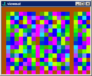
Remembering Euler's Theorem, we would expect every element, raised to the totient power, to output 1. Indeed, the arrays above show columns of 1s five columns in from the right, in the totient power position.
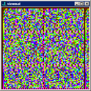
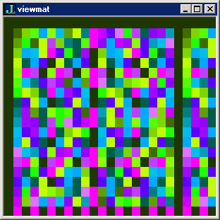
J can help us find such patterns with viewmat, a verb for translating arrays of numbers into arrays of colored cells.