Lecture Four:
Bernoulli Numbers
by Kirby Urner
Oregon Curriculum Network
First posted: Oct 14, 2002
Last updated: Oct 23, 2002
I. BASIC PROGRAMMING
So far, we've been using J in an interactive mode, perhaps saving interim results in variables. When we end the session, our work goes away.
For example, we might define polynomial multiplication in one line, and use it to generate a table:
   mp     =: +//.@(*/)    NB. polynomial multiplication

   1  1 mp^:(i.11) 1      NB. (x+1)^n, powers 0 through 10
1  0  0   0   0   0   0   0  0  0 0
1  1  0   0   0   0   0   0  0  0 0
1  2  1   0   0   0   0   0  0  0 0
1  3  3   1   0   0   0   0  0  0 0
1  4  6   4   1   0   0   0  0  0 0
1  5 10  10   5   1   0   0  0  0 0
1  6 15  20  15   6   1   0  0  0 0
1  7 21  35  35  21   7   1  0  0 0
1  8 28  56  70  56  28   8  1  0 0
1  9 36  84 126 126  84  36  9  1 0
1 10 45 120 210 252 210 120 45 10 1
Typically, however, we'll want to define a verb as a series of programmed steps, and have these verbs invoke one another. And we won't want to redefine these verbs from scratch every time we use them, meaning we'll want to save our code in persistent files.
The interactive execution window is where to test fragments of a longer program, which, once debugged, may be copied to a text window and saved as a runnable file. When the file is run, the operators it defines (verbs, adverbs, nouns, conjunctions) will become available to us in some locale (more on locales another time).
II. BERNOULLI NUMBERS
For example, suppose we'd like to compute the Bernoulli numbers. Several algorithms are available, including one based on the above expansion of (x + 1)^n.
The algorithm for deriving each successive Bernoulli number uses the binomial coefficients in each successive row of Pascal's Triangle, multiplied by all the Bernoulli numbers derived so far, beginning with B[0]=1:
   0 = (2 * B[1]) + (1 * B[0])
   0 = (3 * B[2]) + (3 * B[1]) + (1*B[0])
   0 = (4 * B[3]) + (6 * B[2]) + (4*B[1]) + (1*B[0])
or...
  B[0] =: 1
  B[1] =: (_1r2) * (1 * B[0])
  B[2] =: (_1r3) * (3 * B[1] + 1*B[0])
  B[3] =: (_1r4) * (6 * B[2] + 4*B[1] + 1*B[0])
So one strategy is to collect our Bernoulli numbers in a list, and to use (x+1)^n, with n increasing, to generate the coefficients. Each step of the way, we'll use all our Bernoullis so far, with the binomial coefficients, to generate the next Bernoulli.
Let's look at a single row of the binomial expansion from the table at the top of this page (ignore any zero padding on the right):
1 9 36 84 126 126 84 36 9 1
What we need to do is multiply all coefficients after _9 by the Bernoulli numbers collected so far. Then add the resulting terms and multiply by 1r9. This will give our next Bernoulli number, which we prefix to a growing list.
Here's a program which codifies this algorithm:
mp   =: +//.@(*/)       NB.  polynomial multiplication

   bernoullis =: 3 : 0
coeffs    =. x: 1 1     NB.  beginning coefficients
bns       =. 1          NB.  first Bernoulli
while. y.>0 do.
   coeffs =. 1 1 mp coeffs   NB.  (x-1)^n
   b      =. (- % 1{coeffs ) * (+/ bns * 2}.coeffs)
   bns    =. b,bns      NB.  growing list of Bernoullis
   y.     =. <:y.
end.
bns
)
III. ANALYSIS OF A SHORT PROGRAM
If you've programmed before, your eye will likely pick out the looping structure, bracketed by the while and end statements. Automatically, J assumes y. is the name of the verb's right argument, which in this case is named bernoullis. Were this a dyadic verb, the left argument would be named x. (again, J simply assumes this).
Asking for bernoullis 10 at the command line will initialize y. to 10. After a couple of variable initializations, the loop begins. It contains a decrement-by-1 statement: y. =. <:y. so that each time through the loop, y. gets smaller, and at zero, finally fails the y.>0 test (part of the while statement) and escapes the loop.
Each time through the loop, we move to the next row of coefficients in the binomial expansion of (x-1)^n. The 2nd line in the loop is the most complicated, and implements the algorithm specified above. Let's look at its details:
coeffs =. 1  9 36  84 126 126  84  36  9  1

b =. (- % 1{coeffs ) * (+/ bns * 2}.coeffs)
The first parenthesized expression takes element 1 of coeffs. Given zero-based indexing, this would be the 9 if coeffs were as shown above. This element (9) is then reciprocated (%) and negated (-), giving _1r9. The result is in rational format because our coefficients were initialized as x: 1 1 before the loop started, meaning all subsequent polynomial multiplications have continued to use extended precision format.
The second parenthesized expression uses dyadic curtail (}.) to take all but the first two elements of coeffs, i.e. in this case: 36 84 126 126 84 36 9 1. These terms are multiplied by the corresponding eight elements in bns, and the results are summed (+/).
Both of these expressions are then multiplied together, giving our next Bernoulli number b. This local variable b is then prefixed to bns in the next line, y. is decremented by one (<:), and the loop begins another iteration.
When we finally escape the loop, bns is what gets returned by this verb (whatever is on the last line constitutes the return value). bns contains a list of Bernoulli numbers in reverse order, i.e. the last Bernoulli computed begins the list.
   bernoullis 10
5r66 0 _1r30 0 1r42 0 _1r30 0 1r6 1r2 1

   bernoullis 11
0 5r66 0 _1r30 0 1r42 0 _1r30 0 1r6 1r2 1
Note that odd-indexed Bernoulli numbers are 0, after the first, which is _1r2.
If we want the nth Bernoulli number, we can just take the first element of what's returned, using head ({.):
   load 'd:\program files\j501a\user\projects\berns.ijs'

   {. bernoullis 50   NB. 50th Bernoulli number
495057205241079648212477525r66
We could also codify this as another verb:
   bernoulli =: 3 : '{. bernoullis y.'

   bernoulli 20   NB. 20th Bernoulli number
_174611r330
IV. PARTS OF SPEECH
Also in need of explanation in the above programs, is the use of the number 3, or the expression 3 : 0, at the outset of a verb's definition.
This 3 is one of four possible values, 1, 2, 3 or 4, and it refers to the part of speech that's being defined. 1 signifies an adverb, 2 a conjunction, 3 a monadic verb with an optional dyadic meaning, and 4 an exclusively dyadic verb.
The : 0 after the 3 indicates that the rest of the definition follows on subsequent lines, until a concluding right parenthesis, alone on a line, is reached. In place of this 0, the complete definition enclosed in single quotes, may be provided on a single line. This was the approach taken in our definition of bernoulli.
V. BERNOULLI POLYNOMIALS
What might we do with Bernoulli numbers?
Originally, they were developed, not by Jakob Bernoulli (1654-1705), but by Johann Faulhaber (1580-1635) writing in 1631. Johann wanted to find the sum of the first n-1 consecutive integers all to the kth power, e.g. 1^4 + 2^4 + 3^4 ... + 100^4. Let's compute the answer using J in simple calculator mode:
   +/ (i.>:100x)^4       NB. i.e. 1^4 + 2^4 + ... + 100^4
2050333330
This sum may be expressed in terms of the 5th Bernoulli polynomial, the coefficients of which are comprised of the first five Bernoulli numbers weighted (multiplied) by the binomial coefficients k ! 5 (k=1...5).
   bcoeffs =: 3 : 0
k        =. x: y.
binomial =. (i.>:k) ! k  NB. binomial coefficients
coeffs   =. binomial * bernoullis k
)
The polynomial we seek, giving the sum of the first n-1 consecutive integers to the kth power, is comprised of the k terms of the k+1 Bernoulli polynomial, multiplied by 1/(k+1). A prefix of 0 ensures that our coefficients align with corresponding powers, i.e. the last term aligns with n^5.
   ] b5 =: 0, }. bcoeffs 5
0 _1r6 0 5r3 _5r2 1

   ] coeffs =: 1r5 * b5
0 _1r30 0 1r3 _1r2 1r5

   coeffs p. 101  NB.  note agreement with above answer
2050333330
And if the question were about consecutive integers to the 10th power, we would use Bernoulli numbers to get the coefficients of the 11th degree polynomial, and so on.
Computing the sum of the first 1000 integers to the 10th power would look like this:
   (1r11 * 0,}.bcoeffs 11) p. 1001
91409924241424243424241924242500


   +/ (>:i.1000x)^10   NB. checking the result
91409924241424243424241924242500
Suppose we'd like to accomplish this step of building the summation polynomial in code. For example, if we wanted the polynomial for the sum of k powers of n-1 consecutive integers, we could say pk =: k sumpoly and then evaluate pk, already a polynomial. This is a case of defining a noun-modified verb (a kind of adverb) to return a tacit verb.
   sumpoly =: 1 : '(0,}.(% >: x:m.) * bcoeffs >:m.) & p.'

   p4 =: 4 sumpoly  NB. returns a tacit verb

   p4 101           NB. apply returned verb to n=100
2050333330

   10 sumpoly 1001  NB. apply verb to argument all at once
91409924241424243424241924242500
Although the last expression above makes it looks like sumpoly is just a dyadic verb, it's really not, as 4 sumpoly wouldn't be a legal expression if it were. The purpose of sumpoly is to bind the appropriate coefficients as the left argument to the polynomial verb. Remember that & means "bind" or "curry."
The m. is optionally used in place of x. in the definition of sumpoly in order to specify that sumpoly expects a noun for a left argument -- an exception will be raised if something different is passed. The arguments m. and n. stand for left and right nouns, while u. and v. stand for left and right verbs. x. and y. stand for left and right arguments of whatever type.
VI. TAYLOR EXPANSIONS
J knows how to generate the Taylor expansion of many primitive functions. The Taylor expansion of f(x) is a polynomial of increasing powers of x with rational coefficients. Deriving this polynomial involves taking successively higher derivatives of f(x) around f(a). We call it the Maclaurin expansion if a=0.
The verb t. returns the coefficients of this polynomial. It's left argument is the function f, and the right argument is the index of the term we want. Using i.n gives us terms 0 through n-1. For example:
   cos =: 2&o.      NB.  o. is the circular functions verb

   cf  =: cos t. x:i.10  NB.  first 10 Taylor coefficients
1 0 _1r2 0 1r24 0 _1r720 0 1r40320 0

   cf p. 1p1  NB.  use polynomial to get cos(pi)
_0.976022

   cos 1p1    NB.  the discrepancy is significant
_1

   (cos t. i.20) p. 1p1  NB. 20 terms instead of just 10
_1

   cos t. x:20  NB.  the 20th coefficient as a rational
1r2432902008176640000
Note the Taylor expansion of e^x and its derivative (recall p.. from Lecture 2):
   ] e =: (^ t. x:i.10)  NB.  Taylor expansion of e^x
1 1 1r2 1r6 1r24 1r120 1r720 1r5040 1r40320 1r362880

   p.. e  NB. given an endless expansion, p.. e equals e
1 1 1r2 1r6 1r24 1r120 1r720 1r5040 1r40320
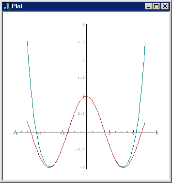
The graph below shows the cosine curve (red) plotted with the curve generated by the first 10 terms of the Taylor expansion of cosine (green).
   load 'plot'

   x =: 0.1*i:50

   ] cf  =: cos t. x:i.10
1 0 _1r2 0 1r24 0 _1r720 0 1r40320 0

   plot x;>(cf p. x);cos x
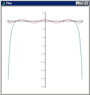
This next graph shows the cosine curve (red) plotted with a Taylor expansion of cosine to 15 terms. Notice the curves coincide over a much broader range (note also the difference in scale between the two graphs).
   x =: 0.1*i:100
   cf2  =: cos t. x:i.15
   plot x;>(cf2 p. x);cos x
Confirmation that e^(i x) = cos x + i sin x may also be obtained by generating the Taylor expansions of both sides:
   f =: ^@(0j1&*)           NB.  f(x) = e^(i x)
   g =: cos + (0j1&*@sin)   NB.  g(x) = cos(x) + i sin(x)

   f t. i.7  NB.  Taylor expansion (to 7 terms) of f(x)
1 0j1 _0.5 0j_0.166667 0.0416667 0j0.00833333 _0.00138889

   g t. i.7  NB.  ditto for g(x)
1 0j1 _0.5 0j_0.166667 0.0416667 0j0.00833333 _0.00138889
The Bernoulli numbers may be generated from the Taylor expansion of the
function
Using 1: allows us to think of the verb train ^ - 1: as a fork, instead of writing <:@^ (i.e. decrement exp(x) by 1). Then the initial dyadic % "hooks" x, to make it the numerator as well. Let's look at the Taylor expansion of this function:
   (% ^ - 1:) t. x:i.11  NB.  Taylor expansion of x/(e^x-1)
1 _1r2 1r12 0 _1r720 0 1r30240 0 _1r1209600 0 1r47900160

   (% <:@^) t. x:i.11    NB.  an alternative expression
1 _1r2 1r12 0 _1r720 0 1r30240 0 _1r1209600 0 1r47900160

   |. bernoullis 10  NB. reverse order to give B0,B1,B2...
1 _1r2 1r6 0 _1r30 0 1r42 0 _1r30 0 5r66

   (|. bernoullis 10) % (! x:i.11) NB. compare with above
1 _1r2 1r12 0 _1r720 0 1r30240 0 _1r1209600 0 1r47900160
What the above lines demonstrate is the the coefficients of the Taylor
expansion of
This pattern of k! occuring in the denominator of a Taylor expansion is part of its definition, and the verb t: (note colon), produces what's called the "weighted Taylor" expansion, meaning successive terms 0...k are automatically multiplied by k!. So t: gives us the Bernoulli numbers directly.
   |. bernoullis 14        NB.  Bernoullis 0 through 14
1 _1r2 1r6 0 _1r30 0 1r42 0 _1r30 0 5r66 0 _691r2730 0 7r6
   (% ^ - 1:) t: x:i.15    NB.  ditto
1 _1r2 1r6 0 _1r30 0 1r42 0 _1r30 0 5r66 0 _691r2730 0 7r6
Given we have direct access to the Bernoullis in this weighted Taylor expansion, it might seem that our earlier algorithm based on binomial coefficients is redundant. However, you'll discover that finding the 100th Bernoulli number using the Taylor expansion takes significantly longer than the binomials-based approach.
However, J does come with a module (./system/packages/math/numbers.ijs) which includes a Bernoulli numbers algorithm that's faster yet, based in turn on so-called tangent numbers.
- Official J website
- Jiving in J
- Introductory J Lectures: [1][2][3][4]
- Java applet re Taylor Expansion by Masashi Sakurai
- Trends in Early Math Education